Ever since its introduction in the 2017 paper, Attention is All You Need, the Transformer model architecture has taken the deep-learning world by storm. Initially introduced for machine translation, it has become the tool of choice for a wide range of domains, including text, audio, video, and others. Transformers have also driven most of the massive increases in model scale and capability in the last few years. OpenAI’s GPT-3 and Codex models are Transformers, as are DeepMind’s Gopher models and many others.

About a year ago, I started working on the Interpretability team at Anthropic, trying to reverse-engineer models in this family. Our goals is to ultimately understand just how these models implement their impressive capabilities; ideally, we aspire to be able to articulate and describe in detail the algorithms that are being executed inside the massive parameters of these models.

Reverse-engineering a model  🔗︎

In some ways, the project of circuits-style interpretability is similar to reverse-engineering a large unknown binary for which we lack source code. We can trace “execution” of a model step-by-step and observe the weights and activations at every point, but what we want is to extract higher-level human-comprehensible algorithms and names which describe what the model is actually doing with those low-level details, in a way that is useful for helping humans predict the behavior of these models.

My background is as a software engineer, and I’ve also done some reverse-engineering work in the past, so I tend to – among other lenses – think of Transformer models through very “computational” or “software engineering” lenses.

This post is an attempt to present the Transformer architecture in a way that highlights some of the perspectives and intuitions that view affords. We’ll walk through a (mostly) complete implementation of a GPT-style Transformer, but the goal will not be running code; instead, I’m going to use the language of software engineering and programming to explain how these models work and articulate some of the perspectives we bring to them when doing interpretability work.

This post is probably best read alongside traditional presentations of these models; I’ve glossed over a lot of details to focus on the pieces I find interesting. The Illustrated Transformer is one great resource, although note we’ll be looking at “Decoder-only” models with only the “decoder” stack, and no “encoder”.

I hope for this post to be a helpful introduction to the details of the Transformer model for anyone with a SWE background who is in the process of getting into ML, and for it to be particularly helpful if you’re looking to do interpretability work.

If you want to follow along, you can find all the code in the post on github.

The Transformer Model  🔗︎

We’ll start with some hyperparameters. I’ve picked the values from GPT-3 175B for concreteness but these can vary across many orders of magnitude. We’ll explain these as needed so don’t worry if you don’t recognize all of them right now.

You can compare these to Table 2.1 in the GPT-3 paper.

(All the code in this post will be in Rust. I’ve tried to avoid using any overly esoteric features, so hopefully it will be somewhat readable even if you aren’t comfortable with Rust in particular)

const N_LAYERS: usize = 96;
const D_MODEL: usize = 12288;
const D_MLP: usize = 4 * D_MODEL;
const D_HEAD: usize = 128;
const N_HEADS: usize = D_MODEL / D_HEAD;
const N_VOCAB: usize = 50000;

Autoregressive language modeling  🔗︎

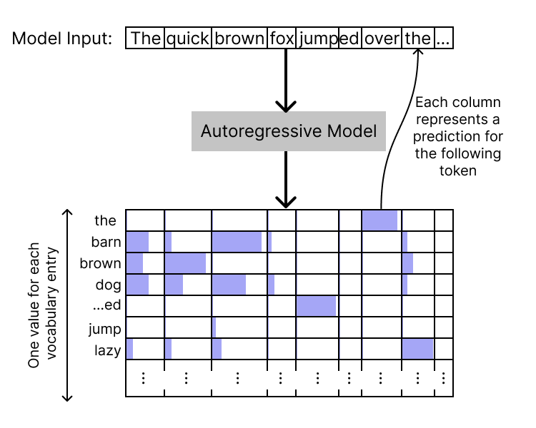
At the highest level, an autoregressive language model (including the decoder-only Transformer) will take in a sequence of text (which we’ll refer to as a “context”), and output a sequence of “logits” the same length as the context. These logits represent, at each position, the model’s prediction for the next token. At each position, there is one logit value per entry in our vocabulary; by taking a softmax over the logit vector, we can get a probability distribution over tokens.

The logits for the final input position thus correspond to predictions for the next token following the context; by sampling from this distribution we can generate a continuation of the context. This method (with various variations) is how Transformers can be used to generate text.

type Token = u64;
type Logits = [f32; N_VOCAB];

trait ARModel {
    fn apply(&self, tokens: &[Token]) -> Vec<Logits>;
}

The residual stream “state vector”  🔗︎

The core internal architecture of the Transformer is a stack of identically-structured layers. Each layer takes in the previous “hidden state” of the model — one state per each token position — does some computation, and then updates that state to produce the following state.

In a Transformer, this “state” is just a vector of floating-point values, one vector for each position, each vector of length D_MODEL. We’ll define a type to hold that state:

#[derive(Clone)]
struct State([f32; D_MODEL]);

// At every point inside the model, we have one State per token
// position
type ResidualStream = [State];

I often like to think of the state (which we call the “residual stream”) as an “opaque data structure.” It contains within it many different features, but those features are opaque and cannot be directly accessed. Instead, the state exposes two main operations:

• We can query it. To do this, we provide a “query” vector, and take a dot product with that vector to produce a single floating-point value.
• We can update it, by providing an “update” vector which will be added to the state vector.

We’ll define type aliases for those types to help keep them straight in our presentation. They’re both the same physical type as the state vector, but we’ll often think of them pretty differently. We’ll also define the basic operations on them.

type Query = State;
type Update = State;

impl State {
    fn zero() -> Self {
        State([0.0; D_MODEL])
    }

    fn update(&self, right: &Update) -> State {
        let mut out = self.clone();
        for (i, r) in right.0.iter().enumerate() {
            out.0[i] += r;
        }
        out
    }

    fn query(&self, right: &Query) -> f32 {
        dot(&self.0, &right.0)
    }
}

fn dot<const N: usize>(l: &[f32; N], r: &[f32; N]) -> f32 {
    let mut out = 0.0;
    for (i, r) in r.iter().enumerate() {
        out += l[i] * r;
    }
    out
}

It’s worth saying a few words about these definitions and how I’m trying to use them to convey intuitions and mental models I have.

• Because of the way layers can only update the state by adding an Update into it, and not by replacing the entire thing, I often think of the Transformer as a “functional program” implemented on a very unusual machine. We pass the state stream through and repeatedly update it to produce to a new state, but we never mutate it in-place or completely throw it away. In this model, we might think of the “model architecture” and the layers as the “instructions” for our weird machines, and the weights as our “operands” for those instructions.
• We will shortly end up with vectors of States, one per token position. Traditionally we represent these directly as 2d tensors (3d with a batch dimension); by defining a State alias we can make it clearer when to think of a 2d tensor as a vector of 1d states, vs as a 2d matrix encoding some linear transformation.
• The “opaque” state and the “query” and “update” operations get at the fact that the residual stream state vectors have no privileged basis space. We should not expect the individual dimensions of the state vector to have meaning, and so we abstract them out.
• Along that line, it’s a quirk of high-dimensional spaces that in N-dimensional space you can construct exponentially-many “almost-orthogonal” vectors (which all have very small pairwise dot products). We suspect Transformers use this property to (noisily) encode far more than D_MODEL features into the residual stream, and I think the “opaque structure you can query for the presence of a particular direction” fits well with this model.

The layers  🔗︎

Now we move to the actual layers of the model. A Transformer work starts with an embedding layer, followed by some number of blocks (which we refer to as “residual blocks” or “resblocks”), and finally an unembedding layer.

struct Transformer {
    embedding: Embedding,
    layers: [ResBlock; N_LAYERS],
    unembedding: Unembedding,
}

The (un)embedding  🔗︎

The purpose of embedding and unembedding is to convert between tokens to and from the internal state. We’ll define them for the standard construction of Transformers that act on tokenized text streams; however, we could also construct models that work on images, audio, or just about anything else pretty much solely by swapping out the (un)embeddings.

The embedding is simply a table containing the initial state vector for each possible token. Applying the embedding is simply an array index:

struct Embedding([State; N_VOCAB]);

impl Embedding {
    fn apply(&self, tok: Token) -> State {
        self.0[tok as usize].clone()
    }
}

Note that, mathematically, indexing into a 2d array like this is equivalent to a matrix multiply with a “one-hot” vector, so you’ll sometimes see this operation described in papers as a matrix multiplication.

We also see here one of the reasons I’ve opted for a named “State” type, in practice. The embedding is physically a 2d D_MODEL x N_VOCAB matrix, and is usually written that way, but I find it much more natural most of the time to think of it as a 1d lookup table of these opaque state objects. This avoids, for instance, any confusion about which axis to index your tensor over.

Of course, it’s also often useful to view it as a matrix so that we can multiply it by other matrices for various analyses: true fluency requires being able to hold both perspectives and move between them.

The unembedding, at the end of the model, is responsible for turning the state back into logits. Typically this is also represented as a matrix of shape D_MODEL x N_VOCAB, and it is applied to a state via a matrix multiplication. This is computationally efficient and mathematically nice, but I’ve opted for a slightly different view:

struct LogitFn(Query);
impl LogitFn {
    fn apply(&self, st: &State) -> f32 {
        self.0.query(st)
    }
}

struct Unembedding([LogitFn; N_VOCAB]);

impl Unembedding {
    fn apply(&self, state: &State) -> Logits {
        let mut out: Logits = [0.0; N_VOCAB];
        for (i, f) in self.0.iter().enumerate() {
            out[i] = f.apply(state);
        }
        out
    }
}

Each vocabulary element has a LogitFn which converts the state into a single floating-point value, by querying the state according to some particular query. To compute the overall logit vector, we simply apply each vocab entry’s query.

This formulation is mathematically identical to the standard matrix multiply formulation. I choose this presentation to emphasize a few points:

• The computation of each individual logit is independent of the others; there are no cross-interactions at this stage of the computation. We’ll get cross-interactions once we apply the softmax, but not in the logit computation.
• The logit computation uses our standard “query” operation; that really is the main way the model looks at the residual stream.
• As with the embedding, I find it useful to be able to move between a view of an NxK matrix as any of:
  • A 2d array of floating-point numbers
  • A linear transformation from K-dimensional space into N-dimensional space.
  • A 1d array of K-dimensional vectors
  • A 1d array of linear functions from K-dimensional space to scalars

(and of course, we can transpose or multiply on the other side, and thus flip the roles of N and K in any or all of the above statements!)

This presentation emphasizes the last two views, which are less frequently spelled out.

The residual blocks  🔗︎

The meat of the transformer is the N_LAYERS “residual blocks,” which happen one after another in between the embedding and the unembedding. Each block consists of an attention layer, followed by an MLP layer.

struct ResBlock {
    attn: AttnLayer,
    mlps: MLPLayer,
}

Let’s take each in turn.

Attention  🔗︎

Transformers use “multi-headed” attention; each attention layer consists of a number of different attention heads operating a smaller subspace of size D_HEAD. Each head is made up of four different (linear) functions:

struct AttnLayer {
    heads: [AttnHead; N_HEADS],
}

type AttnVector = [f32; D_HEAD];

struct AttnHead {
    W_Q: Box<dyn Fn(&State) -> AttnVector>,
    W_K: Box<dyn Fn(&State) -> AttnVector>,
    W_V: Box<dyn Fn(&State) -> AttnVector>,
    W_O: Box<dyn Fn(&AttnVector) -> Update>,
}

I’ve chosen to completely abstract the Q, K, V, and O weight matrices as generic functions from the relevant domain into the relevant range. We’ll remember, though, that we don’t actually mean “arbitrary function” here, but rather “arbitrary linear function,” aka “matrix.”

I like this representation because it helps me keep straight the separation between the “entire self-attention operation” – which includes the Q, K, V, and O projections – and the “core attention” operation which uses the resulting vectors. It also emphasizes that we want to think of these weights not just as arbitrary bags of floating-point numbers, but as operations that transform between different vector spaces. The type signatures also make it very clear that W_O is of a different type than W_Q, W_K, and W_V.

Attention is the only operation that mixes information between token positions. Thus, methods on AttnHead and AttnLayer will operate on a &[State] instead of a single State object. I find this convention very helpful for keeping straight which parts of the Transformer operate across multiple positions, and which ones are local to a position. I love it when we can use a type system to make properties like this more obvious to a reader of our code.

Attention heads are probably the most complex component in a Transformer. I’ll present the code with heavy commenting inline to try to explain what’s going on.

impl AttnHead {
    fn apply(&self, states: &[State]) -> Vec<Update> {
        // Apply the Q, K, and V projections to produce Q, K, and V
        // vectors for each token position.
        let qs: Vec<AttnVector> = states.iter().map(&self.W_Q).collect();
        let ks: Vec<AttnVector> = states.iter().map(&self.W_K).collect();
        let vs: Vec<AttnVector> = states.iter().map(&self.W_V).collect();

        let mut values: Vec<_> = states.iter().map(|_| [0.0; D_HEAD]).collect();

        // Iterate over each token position to compute the output at
        // that position
        for (src, my_q) in qs.iter().enumerate() {
            // Each position may attend to any earlier position. We
            // compute an attention "score" between the current
            // position and each earlier position by dot-producting
            // our Q vector with their K vector.
            let mut scores = Vec::with_capacity(src);

            let visible_indices = 0..=src;

            for i in visible_indices.clone() {
                scores.push(dot(my_q, &ks[i]));
            }

            // We use a softmax to turn that vector of scores into a
            // probability distribution
            softmax(&mut scores);

            // Now we loop over each visible position again, weight
            // their V vector by their attention weight, and sum them
            // all together.
            for i in visible_indices {
                let score = scores[i];
                let v = vs[i];
                for (j, vj) in v.iter().enumerate() {
                    values[src][j] += vj * score;
                }
            }
        }

        // Now we have a value vector for each position. Use the O
        // projection to project it up to a full State vector
        values.iter().map(&self.W_O).collect()
    }
}

I’ve chosen to write the actual “attention” operation as an explicit loop over “source” positions. In most presentations this is written in a more vectorized form, with a mask to encode the “autoregressive” or “causal” property that tokens can only “see” to earlier tokens.

Here, again, I go back and forth between different perspectives, but I do often find it easiest to reason about attention from the perspective of a single source position at a time, and only then efficiently vectorize it in my ML framework; and I think this perspective aligns well with that view.

An attention layer just applies each attention head, and sums their outputs:

impl AttnLayer {
    fn apply(&self, states: &[State]) -> Vec<Update> {
        let mut updates: Vec<Update> = states.iter().map(|_| State::zero()).collect();

        for h in self.heads.iter() {
            let head_out = h.apply(states);

            updates = updates
                .iter()
                .zip(head_out.iter())
                .map(|(l, r)| l.update(r))
                .collect();
        }

        updates
    }
}

I’ll make a few observations about this formulation:

• I use a lot more explicit loops and indexes than in the usual mathematical notation, which lets us elide a lot of details down into nice Σ expressions, matrix multiplies, and such. The math is very convenient and expressive once you get fluent with it, but I also like having a more explicit version available in my head. I also think I would have found this presentation helpful when I was first understanding Transformers, just because it’s written in a language I’m already fluent in.
• Notice that all of the “computation” in an attention head happens in the lower-dimensional AttnVector space. I mentioned earlier that I like to think of the State vector as an “opaque type”; in that lens, the Q, K, and V projections act as “accessors,” retrieving some (head-specific) attributes or features stored in that larger opaque abstraction; we can then do computation on those features, and use the W_O “setter” to tell us how to store the result back into the state vector.
  • If we wanted, we could write (e.g.) W_Q as [Query; D_HEAD] — it projects out D_HEAD queries of the state vector. I chose not to do so because the individual dimensions of queries and keys are also not necessarily meaningful, so I don’t want to overly highlight them.
• This formulation, for me, hints at the fact (discussed in more length in our first paper) that W_Q and W_K interact, and that W_V and W_O interact, but that there’s no direct interactions between the other pairs of matrices (e.g W_Q and W_V). I’ll present an alternate formulation of attention later, which is impractical to implement, but makes this observation explicit.

MLP Layers  🔗︎

By comparison, an MLP layer is almost trivial. MLP layers are usually written as parameterized by two matrices, sometimes called W_in and W_out, or W_up and W_down. I’ve chosen instead to emphasize the computational structure of those matrices by phrasing a layer as a list of individual “neurons”; each neuron in turn has an “input” and “output,” using our Query and Update types.

Each neuron then has a very simple operation:

• It queries the state using its input vector, to produce a single scalar.
• It applies a nonlinear function to that scalar (this is typically ReLU or GeLU, although other options exist)
• It then scales its output vector by that scalar.

The MLP layer as a whole applies each neuron in parallel, and sums the result.

Typically we’d think of the activation function as a property of the entire Transformer, not each layer, and use one consistent activation function. I’ve compromised here and put it on the layer because it makes the code nicely self-contained.

struct Neuron {
    read: Query,
    write: Update,
}

struct MLPLayer {
    mlps: [Neuron; D_MLP],
    nonlinear: fn(f32) -> f32,
}

impl MLPLayer {
    fn apply(&self, state: &State) -> Update {
        let mut out: Update = State::zero();
        for mlp in self.mlps.iter() {
            // "act" is for "activation", a pretty standard naming
            // convention
            let pre_act = mlp.read.query(state);
            let post_act = (self.nonlinear)(pre_act);
            let unit_out: Update = State(mlp.write.0.map(|f| f * post_act));
            out = out.update(&unit_out)
        }
        out
    }
}

We note, once again, that the types immediately clarify that MLPs only happen to one position at a time.

I find this presentation somewhat helpful for clarifying and demystifying MLP layers. It makes it clear that each neuron acts completely independently, and also that the operation of each individual neuron is almost trivial in its simplicity: a dot product, a nonlinearity on a single point, and then a multiply-accumulate of an output vector. The complexity of the MLP layer comes entirely from the aggregation of all of these individual effects.

As with everything else in this document, I find the real value comes from having multiple perspectives that I can pivot between as needed. Treating the input and output projections as matrices or linear transformations exposes a lot of rich structure that we can’t readily talk about in this “computational” view.

Putting it all together  🔗︎

We’re now ready to implement the full Transformer. At this point it’s mostly ceremony, but we’ll include it for completeness:

impl ARModel for Transformer {
    fn apply(&self, tokens: &[Token]) -> Vec<Logits> {
        // Embeddings: convert tokens into initial states
        let mut states = tokens
            .iter()
            .map(|t| self.embedding.apply(*t))
            .collect::<Vec<_>>();

        // Pass the hidden state through each layer in turn
        for layer in self.layers.iter() {
            let attn_out = layer.attn.apply(&states);
            states = states
                .iter()
                .zip(attn_out.iter())
                .map(|(l, r)| l.update(r))
                .collect();

            for i in 0..states.len() {
                let mlp_out = layer.mlps.apply(&states[i]);
                states[i] = states[i].update(&mlp_out);
            }
        }

        // Then apply the unembedding to get out logits
        states.iter().map(|s| self.unembedding.apply(s)).collect()
    }
}

Simplifications and Omissions  🔗︎

I’ve left a few important details out of the model, either because there’s no single standard implementation, or because I felt they would distract from the core takeaways. Consult an actual implementation (such as HuggingFace’s or GPT-NeoX) if you want to actually build and run a Transformer. But I’ll mention some of the pieces I left out here.

Positional Encodings  🔗︎

Astute readers might have noticed that our implementation contains no positional information; the attention operation sees all earlier positions and has no mechanism to know which positions are closer to the current token, or any other information about their position.

Real Transformers use any one of a number of mechanisms to give models positional information. I’ll mention two:

• The classic “Attention is All You Need” Transformer added a bunch of sine and cosine waves of varying frequencies directly into the activations just after the embedding. We assume the model will use to distinct subspaces for “content” and “positional” information, and using basic trig functions lets the model learn operations like “subtract 1 from my position” as linear transformations of the “positional” subspace. Consult the exercises from our first paper if you want to work through the details.
• Rotary Attention is an increasingly common choice; it uses a clever transformation on the keys and values in order to effectively implement a relative attention mechanism (where the model sees only relative positions, like “three tokens ago,” instead of absolute positions, like “token index 21”) efficiently and cheaply.

Layer Normalization  🔗︎

Real Transformer implementations use Layer Normalization (or sometimes RMSNorm) either before or in between each layer, in order to aid with stability during training. Proper normalization is critical to stability during training, but adds only a very small amount of computation or additional parameters to the model, so for many purposes we believe it can be glossed over from a conceptual perspective, and I’ve chosen to do so here.

Our team’s first paper includes a few more notes about this choice.

Biases  🔗︎

Transformers often include bias terms following some of the matrix multiplications, which take the term of a single vector of parameters added in following the multiply. This to say, we replace the linear transformations with affine transformations.

In practice, we believe biases not to be terribly important (they, too, represent a small fraction of parameters and computation), and they can always be simulated if desired by keeping one dimension in the residual stream fixed to 1.0 and using that term of our matrices as the constant offset. Thus, I also omit them here for simplicity.

Attention without query, key, or value vectors  🔗︎

In our first paper, we talk about splitting attention heads into two circuits, the “QK” and “OV” circuits. As a bonus — and caveating that this implementation would be even more tragically inefficient than the previous one — I want to show how we would represent that perspective in the model here.

Our alternate attention heads only two fields, one for each “circuit”, with type signatures describing their new functions:

struct AlternateAttnHead {
    W_QK: Box<dyn Fn(&State, &State) -> f32>,
    W_OV: Box<dyn Fn(&State) -> Update>,
}

The implementation is fairly similar, but now we don’t ever materialize queries, keys, or vectors, but operate always in the State space:

impl AlternateAttnHead {
    fn apply(&self, states: &[State]) -> Vec<Update> {
        let mut output = states
            .iter()
            .map(|_| State::zero())
            .collect::<Vec<Update>>();

        // Iterate over each token position to compute the output at
        // that position
        for (src, src_state) in states.iter().enumerate() {
            // Each position may attend to any earlier position. We
            // compute an attention "score" between the current
            // position and each earlier position by applying the QK circuit to both
            // positions
            let mut scores = Vec::with_capacity(src);

            let visible_indices = 0..=src;

            for i in visible_indices.clone() {
                scores.push((self.W_QK)(&src_state, &states[i]));
            }

            softmax(&mut scores);

            // Now we loop over each visible position again, compute
            // the output update using the OV weight, scale it by the
            // attention weight, and accumulate.
            for i in visible_indices {
                let score = scores[i];
                let o = (self.W_OV)(&states[i]);
                let scaled = State(o.0.map(|f| f * score));
                output[src] = output[src].update(&scaled);
            }
        }

        output
    }
}

This main downside to this approach is that it doesn’t expose the key fact that attention takes places in a smaller vector space of size D_HEAD. That fact is both mathematically important (attention can only move a small subspace worth of information, not the entire residual stream), and important to the computational efficiency of attention.

However, even though we would never use an implementation like this, I find it informative to write out as a tool for thought, and I enjoy the exercise of using code as a medium for communication and reasoning to express what would usually be expressed in mathematical notation.

Why is this so inefficient?  🔗︎

Let’s just spell out why this implementation is so much less efficient.

We’ll start by looking at the normal implementation of attention, for reference. We’ll consider a single attention head; for the total work we can just multiply everything by \(n_{heads}\), which will mostly have the effect of changing \(d_{head}\) to \(d_{model}\) everywhere.

We’re also just going to count multiplication operations, for simplicity; in practice this covers essentially all of the relevant work.

• Each of the K, Q, V, and O multiplications is \( d_{head}\times{}d_{model} \). Applying those at every position nets out to \(4d_{model}d_{head} \) operations across all heads.
• Then we have the nested loops over positions. If we have \(n_{ctx}\) positions in our context, there are \(n_{ctx}^2\) pairs of them¹; when people refer to a vanilla Transformer as “quadratic”, this loop is what they’re talking about.
• At each pair of positions, we do the QK dot product (\(d_{head}\) multiplications), and the V*score multiplication (another \(d_{head}\) multiplications). Thus we arrive at \(2n_{ctx}^2d_{head}\) multiplications.
• Summing these terms and factoring out a bit we arrive at

$$2d_{head}n_{ctx}(2d_{model} + n_{ctx})$$

total multiplications for a single attention head. We note that for large models, we generally have \(d_{model} \gg n_{ctx}\) (GPT-3 175B: \(d_{model}=12288\) vs \(n_{ctx}=2048\)), and so the quadratic term actually contributes very little to the computational cost!

However, what if we did the full State operations at every position? For maximum efficiency we would represent W_QK and W_OV in factored form, as a pair of \(d_{model}\times{}d_{head}\) matrices which we multiply in the appropriate order. We would do this operation at each point inside the nested loop, for a total of

$$n_{ctx}^2(4d_{head}d_{model})~~=~~2d_{head}n_{ctx}(2d_{model}n_{ctx})$$

multiplications! Now, instead of \(d_{model}\) and \((n_{ctx}\) adding on the right hand side, they multiply, and our computational cost goes absolutely through the roof. Essentially, what has happened was that the traditional version “lifts” the expensive matrix multiplies out of the inner loop, so that we only have relatively-cheap 1d operations inside the loop. We’ve undone that optimization, and are now doing the much-more-expensive 2d matrix operations inside the inner loop, which is never desirable.

Closing Thoughts  🔗︎

I really enjoyed this writeup. I feel pretty satisfied about this alternate perspective for understanding and thinking about Transformers, and about the use of notation and types to express the some of the concepts I use to think about these models. I’m hopeful this post will be helpful to other software engineers who are interested in getting into or learning modern ML models, especially anyone interested in Transformer interpretability!

If you want to read more, I recommend our transformer-circuits site, where we’ve published our first two papers and some additional resources outlining what we’ve learned and how we think about these models!

Alternately, if this post has left you feeling like you better-understand the Transformer but wanting to check your understanding, I recommend trying to write your own in PyTorch or JAX! You can get a working single-GPU model in very few lines of code, and it’s very cheap to get small amounts of GPU time in Google Colab or TPU time from the Google TPU Research Cloud, even if you don’t have a GPU of your own. Writing a full model end-to-end and watching your loss start to come down is really quite fun.

And, of course, if you’re interested in working with me on these models full time, Anthropic is hiring! We don’t require ML experience for strong software and systems engineering candidates; we tend to be bottlenecked on engineering as much as or more so than on ML expertise, and we’re very happy to help strong engineers learn the ML that they need to in order to be productive here!