(This post is cross-posted from Honeycomb’s instrumentation series).

One of my favorite concepts when thinking about instrumenting a system to understand its overall performance and capacity is what I call “time utilization”.

By this I mean: If you look at the behavior of a thread over some window of time, what fraction of its time is spent in each “kind” of work that it does?

Let’s make this notion concrete by examining a toy example. Imagine we’re running a job that pulls request events off of a distributed queue, and updates a hit count table in a database:

while True:
  req = queue.pop()
  route = compute_route(req)
  db.execute('''
    UPDATE hitcount WHERE route = ? SET hits=hits + 1
    ''', (route, ))
  req.finish()

How should we instrument this? How can we monitor how it is performing, understand why it’s getting slow if it ever does get too slow, and make an informed capacity planning decisions about how many workers to run?

We’re making several network calls (to our queue and to our database) and doing some local computation (compute_route). A good first instinct is to instrument the network calls, since those are likely the slow parts:

# ...
  with statsd.timer('hitcount.update'):
    db.execute('''
      UPDATE hitcount WHERE route = ? SET hits=hits + 1
      ''', (route, ))
  with statsd.timer('hitcount.finish'):
    req.finish()
# ...

With most statsd implementations, this will give you histogram statistics on the latencies of your database call – perhaps it will report the median, p90, p95, and p99.

We can definitely infer some knowledge about this process’s behavior from those statistics; If the p50 on hitcount.update is too high, likely our database is overloaded and we need to do something about that. But how should we interpret a slow p95 or p99? This is a background asynchronous job, so we don’t overly care about the occasional slow job, as long as it keeps up in general. And how do we tell if we’re running near capacity? If it’s making multiple calls, how do we aggregate the histograms into a useful summary?

We can get a much cleaner picture if we realize that we care less about the absolute time spent in each component so much as we care about the fraction of all time spent in each phase of the component’s lifecycle. Is a given worker spending most of its time waiting on the database, or is it spending most of its time idle, waiting for new events?

We can instrument that by counting the total time spent on each operation, and then normalizing to counts-per-second in our stats pipeline, giving us a unitless seconds-per-second ratio. This might look something like this:

@contextmanager
def op(what):
  start = time.time()
  yield
  statsd.increment('hitcount.total_s',
                   value=(time.time() - start),
                   tags=["op:" + what])

while True:
  with op('receive'):
    req = queue.pop()
  with op('compute_route'):
    route = compute_route(req)
  with op('update'):
    db.execute('''
      UPDATE hitcount WHERE route = ? SET hits=hits + 1
      ''', (route, ))
  with op('finish'):
    req.finish()

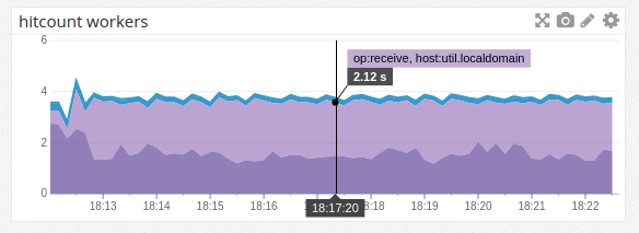
We can now tell our metrics system to construct a stacked graph of this metric, stacked by tags, and normalized to show count-per-second:

Since each worker performs one second per second of work, the graph total gives you the number of active workers (and indeed, I generated this example with four workers). We’re losing a bit of time (potentially in the statsd.increment calls themselves?), but we’re pretty close.

We can immediately see that we’re spending most of our time talking to the database – 2.7s/s or (dividing by 4) about 68% of our time. And the stacked graphs give a very clear visualization of the overall usage of the system.

The above image shows a system at running at capacity. If we’re not, then the graph gives us an easy way to eyeball how much spare capacity we have:

If we’re at capacity, we will never be waiting on messages, and we should be spending nearly no time in the “receive” state (from the above graph, we know that’s not quite true for this toy system; It’s more true in a heavierweight system, and still a good approximation here). Thus, we can treat all the time in “receive” as spare capacity, since that represents idle time when the workers are waiting for new messages to be available, instead of performing work.